| Chapter 4. Computational Procedures | ||
|---|---|---|

|
Part I. AMPAC™ 10 User Guide |  |
| Chapter 4. Computational Procedures | ||
|---|---|---|
|
|
Part I. AMPAC™ 10 User Guide | |
Abstract
This chapter provides a brief summary of some of the more important algorithms found in AMPAC™. A full bibliography is provided in Chapter 17, References.
Table of Contents
Solving for the wavefunction of a molecule is the central activity in quantum chemistry programs. The wavefunction must be obtained at every geometry to compute its energy, gradient, and all other properties. Some computational procedures, particularly for complex procedures like CHN, PATH, or ANNEAL, may require the wavefunction to be computed hundreds or even thousands of times. As such, stability and efficiency in the calculation of the molecule’s wavefunction is very important.
Self consistent field (SCF) represents the fundamental starting point in almost all quantum mechanical methods. (Other methods, such as Configuration Interaction or C.I., start with SCF but then go further.) The most common means of achieving SCF is Roothan’s procedure. It starts with an initial guess for the molecular orbitals (MOs) for the system, which may be created from scratch or taken from a previous calculation. The Fock matrix is constructed from these MOs and then diagonalized to yield a new set of MOs. This is repeated until the MOs are converged. Convergence is when the MOs produced from diagonalizing the Fock matrix are the same as the ones used to produce the Fock matrix and hence are described as being self consistent. This method for solving for the MOs is generally useful but may not converge or may converge very slowly in certain cases. Numerous strategies for improving convergence, such as extrapolation and level-shifting, have been developed to reduce some of these problems.
AMPAC utilizes a very different procedure for solving for the wavefunction. To begin with, any valid set of MOs can be viewed as simply being an orthonormalized set of vectors. The correct MOs are the set of orthonormal vectors that minimize the total energy of the system. Any attempt to minimize the energy with respect to MO coefficients must therefore be constrained to preserve orthonormality. This optimization constraint prevents us from using standard set of optimization algorithms to solve for the MOs. To utilize these standard optimization algorithms, we must first express the problem in terms of variables that automatically maintain the orthonormality of the MOs. The first step, then is to recognize that all possible trial MOs can be expressed as an orthonormal set of vectors (i.e. the current set of MOs) times a general orthogonal transformation matrix. The requirement that the transformation matrix must be orthogonal means that we still have an optimization constraint. This transformation matrix, however, can be expressed as the exponential of a general anti-symmetric matrix. This is further simplified by recognizing that the exponential of a matrix can be rewritten as a highly convergent power series. Applying these substitutions, we can now write the problem as an unconstrained optimization of the elements of a simple anti-symmetric matrix. Standard optimization techniques can now be applied to minimizing the energy.
The actual task of optimizing the electronic variables involves two main classes of methods: pseudo-Newton and Newton. The pseudo-Newton methods utilize the energy and electronic gradient and then build up an approximate electronic Hessian using only gradient information. By avoiding the computation of the exact electronic Hessian, pseudo-Newton methods are generally very fast although they may run into difficulties due to the approximate nature of the Hessian. The Newton approach is more commonly referred to as QCSCF (quadratically convergent SCF) because of its quadratic rate of convergence. QCSCF forms the exact electronic Hessian (expensive), projects it onto a well chosen set of electronic parameters, and then diagonalizes it. Analysis of its eigenvalues determine if the current wavefunction is a minimum or other extremum and so be used to discard spurious SCF solutions. QCSCF is considerably more expensive than the pseudo-Newton methods but is correspondingly more stable and convergent than pseudo-Newton.
AMPAC will generally start by using pseudo-Newton methods and then switch to QCSCF if needed. (Using the keyword QCSCF will force AMPAC to begin with QCSCF.) The pseudo-Newton methods include steepest descent, BFGS, and trust region and AMPAC will automatically switch between them depending on the circumstances. The keyword SCFPRT will show the specific method that was used during that iteration along with information about the SCF convergence. By default, AMPAC allows 200 SCF cycles, of which the first 50 cycles are dedicated to the pseudo-Newton methods. (This default may be changed by using the SCFMAX keyword.) The QCSCF method usually converges any kind of ill-conditioned SCF problem in less than 50 cycles.
As programs in high-level languages like FORTRAN are moved (“ported”) from one system to another, slight discrepancies can arise in some of the calculated values due to different implementation of compilers and architecture. This is to be expected and the differences should be systematic (up to 0.05 kcal/mol on ΔHf and 0.01 kcal/mol/Å on derivatives). On a given computer system these errors must be very small to allow the density matrix (and hence the energy gradients which are highly dependent on the density matrix) to converge. Second order properties such as polarizability and force constants are very sensitive to this lack of convergence and can take on incorrect values if the gradient and wavefunction convergence are not complete. The quality of the density matrix convergence is governed by the SCFCRT parameter. The following table lists the default values of SCFCRT in different situations.
The user may specify convergence criteria by using the SCFCRT keyword. The lower boundary allowed for this value in 1 x 10-13 and is used if SCFCRT=0 is placed on the keyword line.
Two criteria (SELCON and PLTEST) are used to test for SCF convergence, and both must be met before a self-consistent field is achieved.
SELCON is the value of SCFCRT re-expressed in kcal/mol. A lower bound is set on this value based on an internal estimate of the accuracy of the computer. If the difference in electronic energy between any two consecutive iterations drops below SELCON, then the first test is satisfied.
PLTEST is the convergence threshold on the RMS norm of the electronic gradient (in eV/radian). This criterion is not a simple value, but is coupled with the SCFCRT via an empirical equation taking into account the roundoff level and the particular wavefunction in use for the calculation. By relating these two values one obtains smoother and more consistent behavior of the SCF response vs. the SCFCRT criterion used alone. This is required in the frequent cases where the energy appears to be stationary but the density matrix is still oscillating (e.g. molecules with heteroatoms involved in a donor-acceptor bond). With PLTEST, one can obtain a comparable level of self-consistence for both the energy and the density matrix.
The default procedure for geometry optimization is the BFGS modification to the DFP algorithm (for references see Chapter 17, References). This method minimizes a real valued function (in this case the heat of formation, ΔHf) evaluated for the system after each SCF convergence. The following messages are produced when AMPAC achieves geometric convergence:
(Formerly “Herbert's Test”) The estimated distance from the current geometry to the minimum is less than EYEAD. The default value of EYEAD is 0.001.
The RMS gradient norm is less than TOLERG. The default value is 0.1
kcal/mol-1/Å-1 (or
kcal/mol-1/rad-1). If the
keyword GNORM=n.n is specified, then TOLERG is
replaced by the value supplied.
The relative change in the geometry over any two successive iterations has dropped below TOLERX. The default value is 0.0001 Å.
The calculated values of the heat of formation on two successive cycles differ by less than TOLERF. Default value is 0.002 kcal/mol-1.
(Formerly “Peter's Test”) In addition to the TOLERG, TOLERF and TOLERX tests, a second test in which no individual component of the gradient norm is larger than TOLERG must be satisfied. If on three successive cycles this test fails, while all other criteria are met and the heat of formation has dropped by less than 0.3 kcal/mol, then the calculation is stopped after issuing the message:
    THERE HAVE BEEN 3 ATTEMPTS TO REDUCE THE GRADIENT
DURING THESE ATTEMPTS THE ENERGY DROPPED BY LESS THAN 0.3 KCAL/MOL
    FURTHER CALCULATION IS NOT JUSTIFIED AT THIS TIME
AMPAC uses geometric gradients extensively in determining when to terminate calculations and to find search directions. These gradients (first derivatives of energy with respect to atomic position) may be computed either analytically (by taking the derivative of an algebraic equation) or numerically (finite difference, must be requested by the keyword DERINU). Each optimizable geometric parameter is assigned a gradient component (g) and the square root of the sum of the squares of these components defines the gnorm:
The RMS gradient norm is used in the geometry optimization methods and is defined:
In both cases N is the number of optimizable geometric parameters. The RMS gradient norm is used to test whether or not the geometry has been successfully converged by an optimizer. (See GNORM keyword to set this convergence threshold.) The RMS gradient norm is used for geometric convergence because it is size-insensitive. That is, molecules converged to the same gradient criterion (typically 0.1 kcal/mol/Å will a comparable accuracy in the geometry regardless of the overall size of the molecule.
The default procedure for geometry optimization in AMPAC is TRUSTE. (This is a change from earlier releases where BFGS was the default optimizer.) TRUSTE uses a pseudo-Newton approach stabilized by a trust region strategy to optimize the geometry. This method is able to tolerate redundancies in internal coordinates and translation/rotation in the full Cartesian space. TRUSTE minimizes the heat of formation (ΔHf) of the molecule and so is useful for finding minima. TRUSTG is similar to TRUSTE but minimizes the gradient norm and so is useful for searching for transition states or higher order critical points. Statistically, TRUSTE is more robust and twice as fast as BFGS or DFP.
The former default procedure for geometry optimization was the BFGS modification to the DFP algorithm (for references see Chapter 17, References). This method minimizes a real valued function (in this case the heat of formation, ΔHf) evaluated for the system after each SCF convergence.
EF (eigenvector following) minimizes the heat of formation (energy) and can be used to search for minima. TS is related to EF but minimizes the gradient norm and so may be used for transition states. EF and TS are described in more detail in Chapter 9, Eigenvector Following.
LTRD and NEWTON are quadratically convergent optimization methods exclusive to AMPAC. They are very accurate and highly reliable, but are slow for larger systems since they calculate a full Hessian matrix at each step in the optimization. NEWTON minimizes the heat of formation (energy), and LTRD minimizes the gradient norm. The Hessian matrix is usually computed from an analytical-numerical method but a twice-numerical method is used if the keyword DERINU is specified. In both cases, simple forward finite difference or central finite difference (better) is used. An estimated standard deviation value for each eigenvalue is printed. LTRD also computes the components of the vibrational frequencies in terms of the internal coordinates rather than Cartesian coordinates, as is the case with FORCE.
Both methods are usable with either internal coordinates or Cartesian coordinates (see
keyword XYZ) and are insensitive to the
redundancies that might arise in some geometry definition schemes (dummy atoms and/or
translations-rotations). Although not exactly the same as a set of local normal modes, the
eigenmodes (eigenvectors of the Hessian available at each iteration) provide a quantitative
picture of the curvature of the potential energy surface in terms of the coordinates defined
by the user through the geometry definition. A vibrational analysis is carried out at
convergence, providing some or all of the following, depending on the value of PRINT=n, the
Hessian matrix, its eigenvalues and eigenvectors, the vibrational frequencies, ZPE (along
with errors), the Jacobian matrix between the user-defined internal coordinates and the
Cartesian coordinates, the force constant matrix (millidynes/Angstroms) in Cartesian
coordinates, and the weighted force constant matrix (millidynes/Angstroms/amu).
Both methods make use of a mixed optimization strategy employing the steepest descent in the energy or in the gradient norm, the quadratic direction, or hybrid of the two. Also the space may be partitioned according to the signs of the eigenvalues. The inflection points on a potential surface may be local minima of the gradient norm, characterized by an extra zero in the eigenvalues of the Hessian. Such points are usually “attractors” of quadratic methods, but LTRD characterizes them accurately. In contrast, NEWTON avoids these points by biasing the search towards the steepest descent in energy.
All of the methods mentioned above are referred to as local optimizers. That is, the optimizer will search for extrema in the region immediately surrounding the input geometry. These methods are very useful in searching for a specific extremum, where one has some idea of a starting geometry. While these methods are very powerful, they are also limited because they require a considerable amount of user input in the form a reasonable starting geometry. To overcome this limitation, AMPAC provides simulated annealing (see Chapter 13, Simulated Annealing) as a non-local optimizer. A non-local optimizer is an algorithm that will search a large region of the potential energy surface for extrema rather than a small region about a geometry. This is useful when one needs to find a large number of critical points in a region of space, without having to provide information about each one.
A stationary point on a potential energy surface (PES) is a point where the gradient vector (first derivative of energy with respect to atomic positions) approaches zero. Such a point is mathematically described most accurately as a critical point. The behavior of the PES in the vicinity of a critical point depends on the second order derivatives of the energy with respect to the atomic position, i.e. the Hessian matrix. The Hessian matrix, its eigenvalues and eigenvectors, are coordinate-dependent but the signs of the eigenvalues do not depend on a change of the coordinates (as long as the full space is spanned). Thus, it is the signs of the eigenvalues which characterize the nature of a critical point. Mathematically, critical points are classified by the number of strictly negative eigenvalues of the Hessian, called the index of the critical point.
At a critical point with index zero, the energy rises upon movement in any direction with respect to the energy value at the critical point. This set of conditions defines a minimum on the PES, a stable conformation of the system. If one or more eigenvalues of a stationary point are negative, there exist directions where the energy rises as above, and others where the energy decreases. This set of conditions defines a critical point that is no longer a minimum, but something else variously called a “col”, a “hilltop”, a “ridge”, or a “super saddle point”. Among these critical points of various indices, the ones of index 1 play a special role in chemistry as they correspond to the transition states in the Theory of Rate Processes.
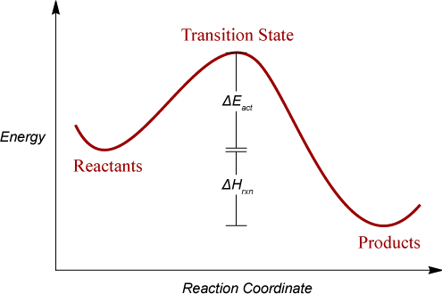
The mathematical description of the energy surface can be related to chemical processes. Reactions are often visualized in terms of an energy profile vs. some chemically important reaction coordinate. The components of this arrangement are shown on the simple (actual PESs may have many degrees of freedom and be multidimensional) figure below. The points labeled correspond to two minima (Reactants, Products) and a maximum (Transition State) and are collectively know as stationary points. Minima on the graph represent stable species on the PES, and are thus stationary points with index 0. The transition state (maximum) on the graph corresponds to a stationary point of index 1. It must be emphasized that these points are the only ones which have mathematically defined properties on the potential graph. Intermediate points on the surface require that some subset of the parameters be constrained, a condition inconsistent with the definition of a stationary point. It should be noted that the semiempirical parameters were derived from molecules at stationary points (minima in fact) and the properties produced by the models are thus only strictly meaningful at these points. However, it has been shown that the chemical model comprising the semiempirical methodologies is valid at positions away from the minima, such as transition states.
Some of the thermodynamic quantities that can be computed by AMPAC and their relationship to the axes of the graph are also presented on the figure. The relationship between kinetics and thermodynamics is well known and the ΔEact (where E is either free energy (G) or enthalpy (H)) is the quantity usually related to kinetics.
The final stage in any calculation is the proper characterization of all results as particular types stationary points. This requires a frequency analysis by LFORCE, HESSEI, FORCE, NEWTON, or LTRD. (Exceptions are CHAIN and CHN, which locate points of index 1.) Ample data exists in the literature showing the danger of not completing this final step in any computational study.[15] For most purposes, LFORCE or HESSEI are to be preferred because only a few of the lowest eigenvalues and eigenvectors are computed in order to establish the specific type of stationary point. FORCE should be used when all of the IR frequencies are desired or if thermodynamic properties are to be computed. Chapter 23, Cartesian Frequencies and Thermodynamics (FORCE) describes this type of analysis using FORCE on the cyclization transition state of 1,3-butadiene. An unrefined gnorm or gradient component indicates that there are residual forces acting on the geometry of the system that must be eliminated before a stationary point is achieved. If FORCE is being used for the frequency computation, a gnorm test is applied and calculation is halted if the value is above 3.0 (see keyword LET). If LTRD is being used and the gnorm is too large, an optimization proceeds using the full Newton algorithm (see the section called “LTRD and NEWTON” for a discussion of LTRD’s function). Chapter 24, Internal Coordinate Frequencies and Gradients (LTRD) demonstrates the use of LTRD.
As mentioned in the last section, if a system has more than one negative eigenvalue, then it is not a transition state, but a point termed variously a “col”, a “hilltop”, or a “ridge” or “super saddle point.” In general, this type of point is near a transition state, and some method must be utilized to optimize to the true transition state. There are several automated techniques in AMPAC for following vibrational modes that aid in this procedure (PATH, EF, TS, and IRC), but this problem can also be solved manually. The basic technique is to determine the atomic motions composing the vibration to be followed, increment the geometry a small amount along these coordinates, and then reoptimize the geometry (gradient minimization).
Finding and characterizing transition states requires some special attention because of their great importance in computational chemistry. Transitions states are extrema with exactly one negative eigenvalue and require gradient minimizers (such as TRUSTG, LTRD, and TS) to find. Transition states are considerably more difficult to find than minima and it is generally more difficult to develop a suitable starting geometry. In addition to the gradient minimizers, there are several other methods that may also be utilized for finding transitions states. The most useful methods for finding transition states are the CHN/ CHAIN methods but these will be described further below. Simulated annealing methods (GANNEAL, TSANNEAL, and MANNEAL) are non-local optimizers and so may find many transition states in the region being searched. The chief drawback of simulated annealing is that it is very costly and is not generally useful for finding a specific transition state. For reactions that correspond primarily to a change in one or two internal coordinates, the reaction path and reaction grid methods respectively can be used. Chapter 25, One-Dimensional Reaction Pathway and Chapter 26, Two-Dimensional Grid Search illustrate the utility of these two methods.
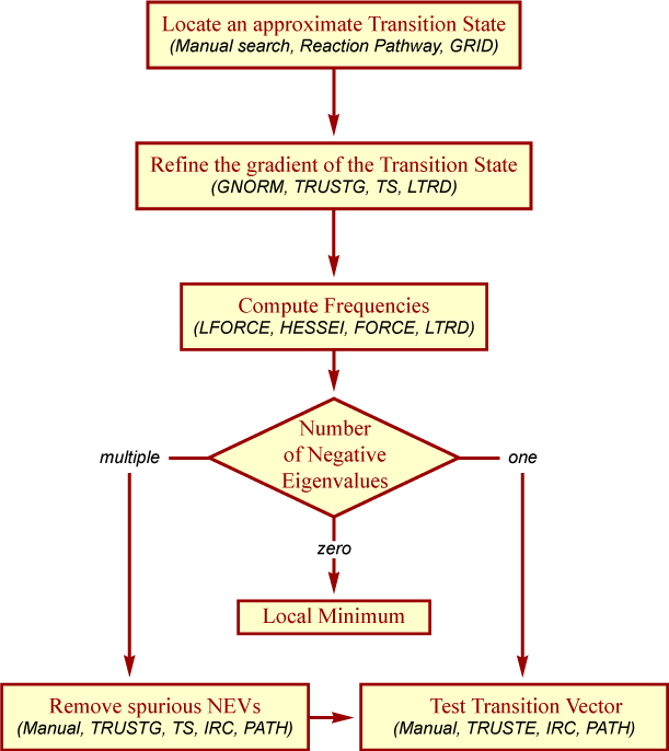
After properly minimizing the gradient, it is important to determine the exact number of negative eigenvalues (NEV) associated with the extrema. The standard method of computing the number of NEV is LFORCE (but also HESSEI, FORCE, NEWTON, and LTRD). If the extremum has zero NEV, then it is a minimum rather than a transition state. If more than one NEV is found, then additional steps must be taken to eliminate all of the extraneous NEV.
Once a genuine transition state has been confirmed, the final step is to confirm that the transition state lies on the pathway between the reactants and products. Starting from the transition state, the transition vector can be followed in both directions until a minimum is reached. This step is critical because it is possible to locate a different transition state than the one that was being searched for. This can be easily done with IRC and PATH using T.V.=1, which will follow the transition vector in both directions to identify both the reactants and products. (The AMPAC GUI can display the resulting pathway running from reactions to transition state to products.) This can also be accomplished manually by incrementing the geometry of the transition state along its transition vector in one direction and then optimizing to a minimum using a standard energy minimizer. The second endpoint can be found by the same procedure but displacing in the opposite direction. (The AMPAC GUI can be very helpful in analyzing vibrations and performing the needed geometry modifications. See Section 2.5 of the AMPAC Graphical User Interface Manual for an example of how this is done.)
The steps for proper refinement and confirmation of a transition state may be summarized as follows:
Because of the great importance of transition states and the inherent difficulties in finding them, AMPAC has a specialized method to overcoming these problems. CHN (or FULLCHN) only requires two geometries along the reaction path that will bracket the transition state. Generally, these two geometries are minima representing the reactants and products respectively. (In the case of dissociated products, a partially dissociated geometry may be preferable to complete dissociation.) By avoiding the need for a guess transition state, CHN avoids one of the greatest hindrances to transition state searches. (CHAIN, the predecessor to CHN, does require a crude guess for the transition state. CHN/FULLCHN only requires the two end point geometries but can take advantage of a guess transition state or additional geometries along the reaction path.)
CHN automates the process of finding a transition state and largely eliminates the complicated multi-step process described in Figure 4.2, “Steps for proper refinement and confirmation of a transition state”. CHN works by generating a series of geometries that form a smooth path between the starting and ending geometries. This chain of geometries is refined with the highest point along the path optimized as the transition state. CHN will automatically compute the number of negative eigenvalues and attempt to eliminate any spurious ones. (If multiple transition states exist along the path, then CHN will locate only the highest one while FULLCHN will locate all of the extrema along the path.) It may still be necessary to use IRC or PATH to verify the reactants and products associated with the transition state. A fuller description of the CHN methods along with examples can be found in Chapter 8, CHN Methods.
Chemists think of molecules in terms of the overlap and combination of atomic orbitals to form molecular orbitals. It is often difficult to analyze the final MOs from an AMPAC calculation based on the output eigenvectors, which are the coefficients of the atomic orbitals. Using LOCALIZE, the occupied eigenvectors are transformed into a localized set of MOs by a series of 2 × 2 rotations which maximize <Ψ4>. The value of 1/<Ψ4> is a direct measure of the number of centers involved in the MO, thus for H2 the value of 1/<Ψ4> is 2.0, for a three-center bond it is 3.0, and for a lone pair it is 1.0. Higher degeneracies than allowed by point group theory are readily obtained. For example, benzene would give rise to a 6-fold degenerate C-H bond, a 6-fold degenerate C-C sigma bond and a three-fold degenerate C-C pi bond. In principle, there is no single step method to unambiguously obtain the most localized set of MOs in systems where several canonical structures are possible, just as no simple method exists for finding the most stable conformer of some large compound. However, the localized bonds generated from this procedure will usually be acceptable for routine applications and more closely follow the chemist’s intuitive expectation.
The concept of a “reaction path” suffers from the lack of a clear definition, in that it has no mathematical form and is coordinate dependent. A reaction path is probably best defined as a special case of a steepest descent path, i.e. a trajectory with the force vector corresponding to the reaction pathway as a tangent. With s (a parameter of integration) and E (the energy as a function of a set of coordinates, x), such a trajectory is defined by the first order system of differential equations:
where wi is defined as a positive weight, e.g. the inverse of the masses of the nuclei.
With s=O as a starting point, a unique trajectory is defined and will always end at a critical point (most of the time, a minimum) when s approaches infinity. The length l of the trajectory from s=O to s=t is given by the following integral along the path:
A unifying definition for the reaction path has been proposed on the basis of dynamics in the limiting case of vanishing kinetic energy. This leads to an opposite-gradient trajectory (steepest descent path), but only within the mass-weighted Cartesian coordinate system. This trajectory defines the intrinsic reaction coordinate or IRC. This definition may also be useful in following steepest descent paths in other coordinate systems. These paths no longer correspond to the IRC, but will end at the same critical point, as the topology of the potential surface is not a function of connectivity.
The PATH method in AMPAC follows such general steepest descent trajectories. This method is often useful for locating weakly stable intermediates along a reaction path or following a spurious eigenmode to refine a transition state. In contrast, the IRC method focuses on the reaction path and the physical properties along it.
A variety of numerical integration algorithms are available in the literature and have been extensively tested in chemical kinetics using semi-classical trajectories. None of the standard methods (Runge-Kutta or Predictor-Corrector) are efficient enough for the integration of a reaction path when a valley (minimum energy reaction pathway, MERP) is followed.
Elsewhere, special integrators have been derived for systems with a large time constant and take the form:
with r a “large” positive number and fi(s) a slowly varying function of s. This is also the case (with fi(s)=O) for a reaction path expressed in the normal modes of a quadratic potential. Anharmonic effects are taken into account by fi(s). Using these properties, a mixed strategy employing both a standard Predictor-Corrector when r is small or negative and an exponential integrator when r becomes large can be derived. This approach does not require that the Hessian matrix (needed for rotation onto the local normal mode basis) be explicitly computed. This condition saves a large amount of computational time and effort. The Hessian is updated using only the gradient evaluations along the path. Such a mixed integrator works much more efficiently than either single standard method when applied to a reaction path expressed in internal coordinates.
(See Chapter 29, Intrinsic Reaction Coordinate (IRC) Calculation and the section called “Integration of a Reaction Path in PATH or IRC” above for a description of the application and underlying theory of IRC.) If physical properties are to be obtained along the reaction path, then IRC should be used. The IRC can be described as a “local normal mode”, immediately related to statistical theories of reaction rates such as transition state theory, RRKM theory, or variational transition state theory. IRC was implemented in AMPAC making extensive use of available materials such as the steepest descent integrator from PATH, the force constants matrix from LTRD, and thermodynamic methods from FORCE. While similar to PATH in many respects, the following differences should be noted:
IRC uses mass weighted Cartesian coordinates even if the geometry is provided in terms of internal coordinates.
IRC explicitly computes the HESSIAN along the path and is more accurate than PATH.
The PATH keyword WEIGHT is inactive with IRC, but an oriented transition vector can be supplied via T.V.
IRC=n.n
can be used to study the properties of points along the reaction path. If
n.n is specified, these properties are computed at each n.n
Å interval. “Transverse” thermodynamic properties are also computed.
The Heats of Formation resulting from AMPAC’s semiempirical calculations are calculated using atomic Heats of Atomization stored in the program. The first step is to calculate the HF total energy of the system as predicted by AMPAC. This is the sum of the CORE-CORE REPULSION ENERGY and the ELECTRONIC ENERGY, both of which quantities are present in the output and archive files. The atomization energy is then computed by subtracting the total energies of the atoms (as predicted by the model being used) in their stoichiometric ratios. The Heat of Formation, ΔHf, of the system can then be calculated using the enthalpies of atomization of the atoms and the atomization energy. While this is not a “true” ΔHf, all of the semiempirical methods in AMPAC were parameterized to experimental ΔHf at 298 K using this formalism.
The standard suite of AMPAC energy minimizers (TRUSTE is the default) is usually sufficient to optimize a given geometry to a minimum on the PES. The performance of these minimizers can fail, however, when the initial geometry provided to the program is near a critical point. An example of this is cyclooctatetraene, which takes on a “bathtub” conformation when optimized in its minimum energy conformation:
However, if the initial geometry is provided as planar (see below), AMPAC minimizers may fail and predict the system to be planar. A frequency analysis (LFORCE or HESSEI) carried out at this point will show one negative eigenvalue, characterizing the geometry as a transition state. In this case the TS corresponds to the process of inversion of the “tub”.
For quasi-Newton methods, such as DFP and BFGS, the entire PES is treated as a minimum, using a definite positive Hessian matrix to determine search direction. The region near a stationary point has a slowly changing gradient and is thus “flat” as far as the search algorithm is concerned. This (coupled with the definite positive Hessian approximation from above) makes this region appear to DFP/BFGS to be a very shallow minimum with an extremely narrow peak corresponding to the actual critical point. Further, if the well is very symmetric, none of the points generated in the search will fall in the very small region of the peak and the search algorithm will not be informed of its existence. Only a full quadratic algorithm such as NEWTON or LTRD will explore the PES in sufficient detail to reveal a problem of this type, (at a large cost in computational effort, as many exact Hessians are computed). Care must be exercised in this region of the PES. The problem can be generally solved by simply introducing a slight degree of asymmetry to the molecule’s definition, allowing it to naturally “roll down the hill.”
|
Copyright © 1992-2013 Semichem, Inc. All rights reserved. |
|
|
 |
|
| Chapter 3. Semiempirical Methods and Parameters |  |
Chapter 5. Presenting Input to the Program |